cuGP

Summary

We have parallelized the training and prediction phases of Gaussian Process Regression on a GPU. We took it a step further and also implemented an approximate algorithm for a distributed setting: DA-cuGP. This version effectively parallelizes all computation across several GPUs in a cluster while also managing light-weight communication between the participating nodes. We were able to obtain significant speedups against strong baselines. Furthermore, to be able to handle arbitrary sized data sets, we extended the approach by adding a decentralized computation-scheduler that appropriately dispatches work across nodes.

Background

Gaussian Process (GP) regression models have become very popular in recent years in the machine learning community. This can be attributed to the flexibility offered by these models to allow users to choose the appropriate covariance function to control the degree of smoothness. GP regression is basically a Bayesian nonparametric model (where an underlying finite-dimensional random variable is replaced by a stochastic process). Formally, a GP is a stochastic process where any finite number of random variables have a joint Gaussian distribution [RW06].

A GP is completely specified by a mean function ($m(\vec{x})$) and a covariance function ($\kappa (\vec{x}_1, \vec{x}_2)$), which for a real process $f(\vec{x})$ can be defined as:

$$ m(\vec{x}) = \mathbf{E}[f(\vec{x})] $$

$$ \kappa (\vec{x}_1, \vec{x}_2) = \mathbf{E}[(f(\vec{x}_1) - m(\vec{x}_1))( f(\vec{x}_2) - m(\vec{x}_2) )] $$

Generally, the mean function is taken as zero. In that case, the covariance function ($\kappa (\vec{x}_1, \vec{x}_2)$) basically turns into the covariance between $f(\vec{x}_1)$ and $f(\vec{x}_2)$. The squared exponential (SE) kernel is a common choice of covariance function (amongst a wide range of available choices for the kernel), and is defined as follows: $$ \kappa (\vec{x}_1, \vec{x}_2) = \exp( -\frac{1}{2l^2} | \vec{x}_1 - \vec{x}_2 |^2 ),$$ where, $l$ is the lengthscale parameter that needs to be estimated.

In order to perform nonparametric regression, a GP prior is placed over the unknown function. The posterior distribution obtained by multiplying the prior with the likelihood is again a GP. The predictive distribution for a new test point ( $ \vec{x}_{t} $ ), given the entire dataset ($N$ tuples of the form $(\vec{x}, y)$) can be shown to be a Gaussian with the following mean ( $ \hat{f_{t}} $ ) and variance ( $ \mathbf{V}[f_{t}] $ ): $$ \hat{f_{t}} = {\vec{k}_{t}}^{T} (K + \sigma_{n}^2I)^{-1} \vec{y} $$ $$ \mathbf{V}[f_{t}] = \kappa (\vec{x}_{t}, \vec{x}_{t}) - {\vec{k}_{t}}^{T} (K + \sigma_{n}^2I)^{-1} \vec{k}_{t} $$ where,

• $K$ is a $N \times N$ matrix where the $ij$th entry is computed as $K_{ij} = \kappa (\vec{x}_i, \vec{x}_j)$,
• $\vec{y}$ is a $N \times 1$ vector formed by stacking the $n$ target values together from the dataset,
• $I$ is a $N \times N$ identity matrix,
• $\sigma^2$ is the noise variance,
• $ \vec{k}_{t}$ is a $N \times 1$ vector where each entry is computed as $ \vec{k}_{t_{i}} = \kappa (\vec{x}_i, \vec{x}_{t})$

In order to learn the different parameters (lengthscale(s) of the covariance kernel, the noise and signal variances), a common technique is to use the marginal likelihood maximization framework (this step can be thought of as the 'training' phase). The log marginal likelihood has the following form:

$$ LML = \log p(\vec{y} | X) = -\frac{1}{2} \vec{y}^T (K + \sigma_{n}^2I)^{-1}\vec{y} - \frac{1}{2} \log |K + \sigma_{n}^2I | - \frac{n}{2} \log 2\pi $$

If we consider $\vec{\theta}$ as the vector of parameters to estimate, gradient based methods (conjugate gradient of L-BFGS) can be employed after obtaining suitable analytic gradients $ \frac{\partial LML}{ \partial \vec{\theta}_i}$.

The main bottlenecks for both training and prediction phases are the compute- and memory-intensive matrix computations, which take $\mathcal{O}(N^3)$ flops, thus limiting the application of GPs for large datasets having $ N > 10000$ samples.

Approach

• Serial implementation

  In order to gain a better understanding of each of the operations involved in both learning (training) and inference (testing) phases, we implemented a serial single-threaded version of the GP regression algorithm. To accomplish this, we implemented our own mini matrix algebra library for all the required operations in GPR. This mini library has routines for Cholesky decomposition, forward substitution, backward substitution among other standard matrix-matrix/matrix-vector operations.

  For maximizing the LML in the training phase, we employed the conjugate gradient solver by Joao Cunha. To be precise, this is the only third party code that we used in our serial implementation, all other routines were written from scratch in C++. Correctness was established by cross-checking outputs of each of the steps with the corresponding results as in the popular GPML framework [RN15] which is written in Matlab.

• GPR on CUDA: First attempt

  After acquainting ourselves with the nitty gritty details at each step, we implemented GP regression on CUDA writing our own kernels for each task. As in the previous case, we implemented the kernels for the required matrix computations ourselves. More precisely, we wrote a recursive blocked version of Cholesky decomposition as described in the paper by Dong et al [DH14]. One of the important steps in computing the likelihood as well as in computing the gradients, is solving a triangular system of equations. An efficient method for solving such a system is to employ forward/backward substitution algorithm. Since both the algorithms are inherently sequential, we implemented a recursive algorithm for efficiently finding the inverse of a lower (upper) triangular matrix as given in [K09]. We also implemented a reasonably fast matrix-matrix multiplication kernel that uses shared memory.

  Implementing the kernels ourselves gave us the opportunity to fuse different operations together. We benchmark our implementation on a synthetic sine dataset, wherein the input data lives in a 10 dimensional space, and the function to approximate is a sine function that depends only on the first dimension. In order to make the targets (function obsrevations) noisy, we add a Gaussian noise to the function values (the variance of this Gaussian is 0.05). Figure 1 shows the performance of the most crucial functions (some of which are implemented with a series of kernels), on the synthetic dataset. Note that all our experiments were performed using the K40 GPUs present in the latedays cluster.

  

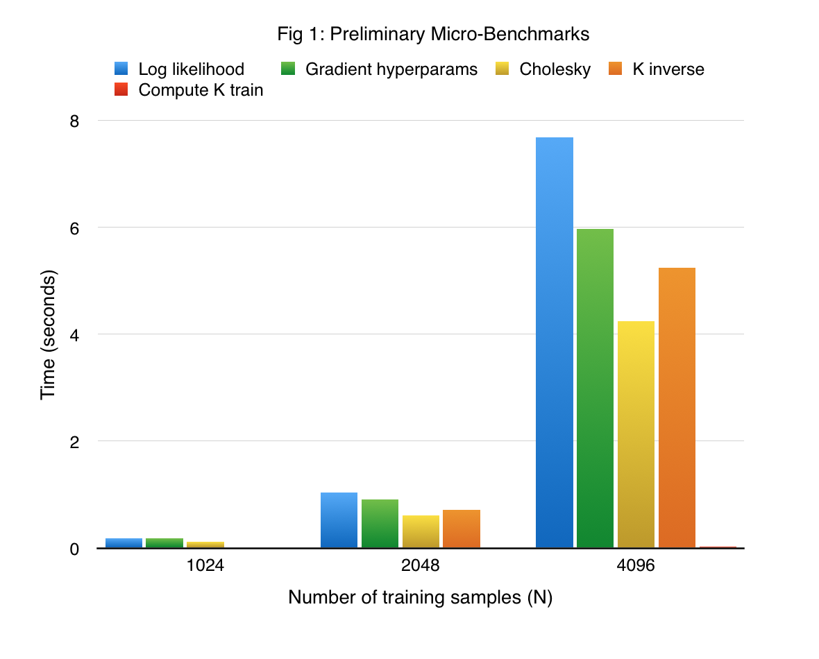
  We see that computation of the gradient of log hyperparameters takes the most amount of time. This is expected because the gradient computation involves an inverse of a lower triangular matrix and generation of the covariance matrix, in addition to vector-vector dot products and matrix-vector dot products and vector-vector dot product. In addition to providing significant insights, this implementation serves as strong baseline for our actual approach.

• cuGP

  For our final approach, we build on the version-1 of our CUDA implemenation. We replaced some of our kernels with routines from cuBLAS/cuSOLVER. More specifically, we employ the following routines from the cuBLAS library:

  • DGEMM for efficient matrix multiplication

  • DGEMV for matrix-vector product

  • DGER: for vector outer product

  • DTRSM: for solving the triangular system of equations.

  For fast Cholesky decomposition, we employ cuSOLVER’s DPTORF routine. Additionally, we use THRUST library routines for vector dot products and parallel reduce. However, we retain our important kernels like the one reponisible for computing the covariance matrix, and another which performs efficient elementwise matrix muliplication, and so on.

  Furthermore, we optimize our other kernels by ensuring low bank contention on memory access conflicts by reading from addresses dictated by the logical location of a thread in the CUDA grid.

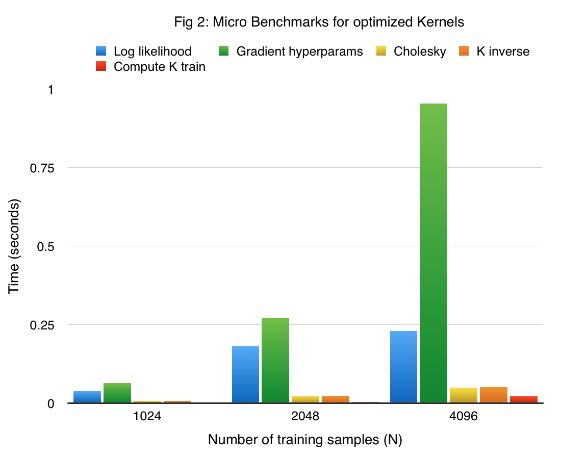
  The performance of the main components in our final single node GP implementation in CUDA of the training phase (referred to as cuGP) is given in figure 2. The results are obtained on the previously described sine dataset.

  
  
  

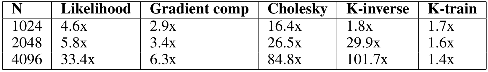
  Considering our earlier approach as a competitive baseline, the speedup obtained with our cuGP implementation for the crucial kernels in our training phase is given in the table below.

  
  

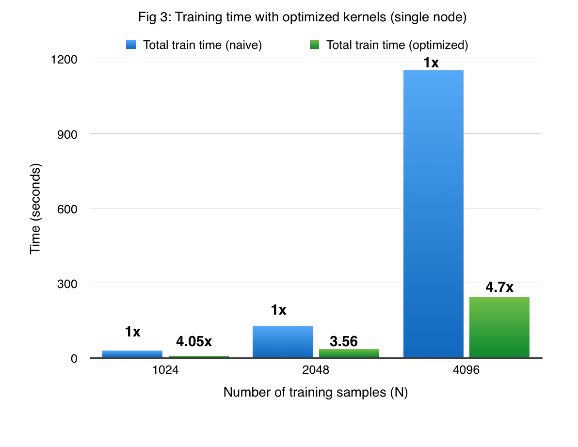
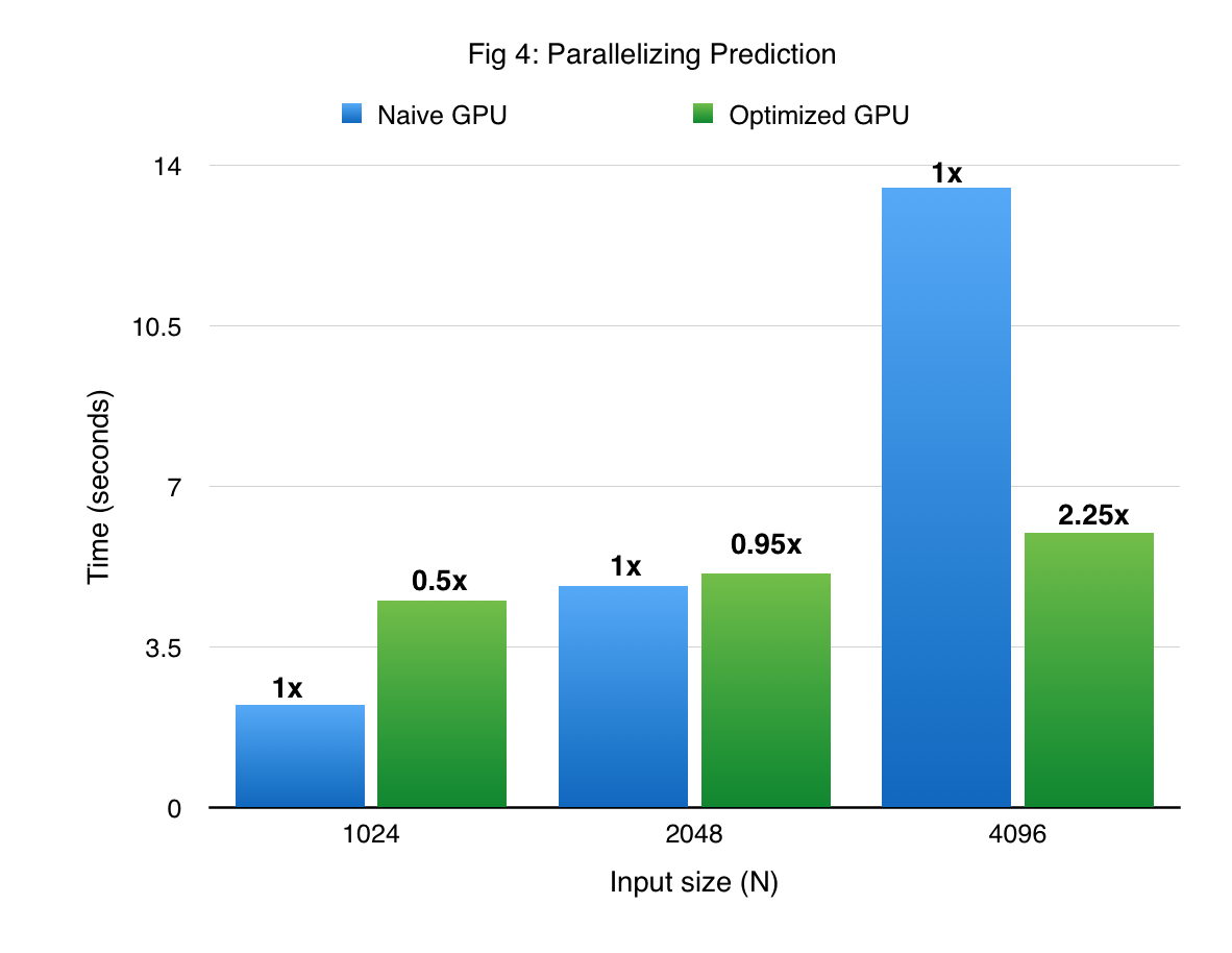
  Figures 3 and 4 compare the performance of cuGP with the baseline in the training and prediction phases respectively. The X-axis shows only the number of training points. In the case of prediction, the number of traning points for each experiment was 1000. We see signifiant speedup values over the baseline for both training as well as testing (prediction) phases. However, for smaller values of the input dataset in the prediction phase (testing phase), the CUDA baseline performs better than cuGP. This is because of the speedup obtained due to fusing of multiple operations in the kernels in the baseline implementation. This makes the baseline better than cuGP, for the testing phase, for a certain range of the dataset size.

  
  
  
  


• DA-cuGP: Distributed Approximate cuGP

  The single node cuGP implementation performs well on datasets of the size $ \mathcal{O}(10^4)$. Howerver, due to the $ \mathcal{O}(N^2) $ storage requirement, the cuGP implementation is limited by the amount of memory available on the device. To further scale, we have implemented a recent approach [DN14] which is an approximation to the exact GP regression. This was our stretch goal up until the checkpoint. We extend the method suggested in [DN14] to multiple GPUs. The high level idea of the approximate approach is to have several "experts", each of which is responsible for a subset of the original data. The approach basically approximates the originial covariance matrix to several blocks. The input dataset is divided into $K$ chunks, and in oursetup each GP expert takes care of a single chunk.

  In this approach, the negative log marginal likelihood can be approximated by the sum of the log marginal likelihood values of each individual expert. The subtle point in the learning (training) phase is that the hyperparameters have to be shared across the experts. Due to this, the time complexity is $\mathcal{O}(N_c^3)$ where $N_c$ is the size of each of the $K$ data shards (in other words, it is basically the data subset size).

  This approach is similar to the parameter-server approach as discussed in the class. So one node (a master node) is responsible for storing the current hyperparamters of the GP model. At each step of the log likelihood / gradient compuatation, each of the workers (experts in our context) need to get the latest value of the hyperparameters, and perform the required computation. The master then collects the partial results and updates the hyperparameters and broadcasts back the new parameters to the experts for the next round.

  We have implemented this approach using mulitple GPUs (which can be thought of as individual experts). In order to communicate the hyper-parameters, we use low-level socket programming for efficiently transferring the information to and from the experts. We tried doing the same using MPI, but we faced some issues in setting up the MPI cluster, and therefore chose to communicate over sockets.

  In our implementation, experts are nothing but nodes on the latedays cluster, each with its own GPU. The host on one of these experts is assigned to be the master, and is responsible for initiating all communication. The other nodes are notified about the identity of the master at program launch. We call our implementation Distributed Approximate cuGP (DA-cuGP).

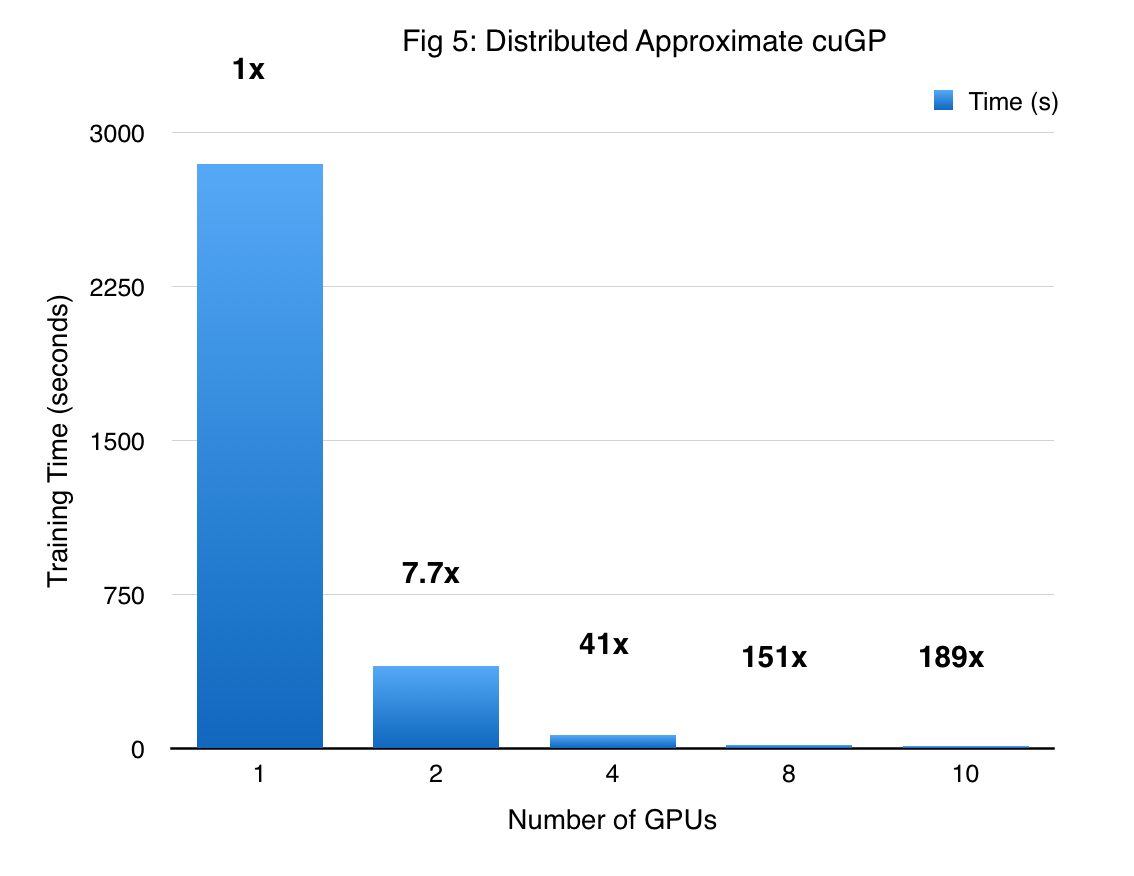
  The performance of the DA-cuGP on the synthetic sine dataset is shown in Figure 5. The first bar corresponds to the exact GP working on a dataset with 10000 points. As we move towards the right, the number of GPUs increases and the size of the dataset per GPU decreases. As one might expect, we obtain massive speedup due to both reduction of the problem size, and asymptotically lower complexity of the approximate method itself. So for 10 GPUs, the shard size is $\frac{1}{10}th$ of that handled by a single GP (which falls back to an exact GP model). Thus, we obtain super-linear speedup since the time complexity of this algorithm scales cubically with the shard size, and this is further amplified by the distributed computation. It is worth noting that as the number of GPUs increase, we incur a higher approximation in the prediction phase. However, inspecting the hyper-parameters we find that the variance in the values is reasonably small.

  
• DAS-cuGP: Distributed Approximate Scalable cuGP

  The size of data that can be handled by DA-cuGP is limited by the number of GPUs available. In order to further scale up, we wrote a decentralized scheduler which can handle arbitary sizes of data. The basic idea is the same - we shard the data into smaller subsets and map each of the shards to the avalable GPUs. Implementing a distributed version of cuGP (DA-cuGP) itself was a stretch goal for us. However, once we implemented DA-cuGP, we realized that it would be interesting to further extend this to a highly scalable version.

  To provide a high level intuition, let’s suppose that we have 8 shards but only 2 GPUs. For computing the log likelihood (LL) at a single step, we require input from all the experts (from all the shards). So the first GPU is assigned to compute the LL for shards 1, 3, 5, 7; and the second GPU computes the LL for the remaining shards (2, 4, 6, 8) in an iterative fashion (it is important to note that only 1 shard can fit in a GPU at one point of time).

  So essentially there is no data locality. But, the tradeoff is that we can now manage greater volumes of data - way more than what can fit even in host memory.

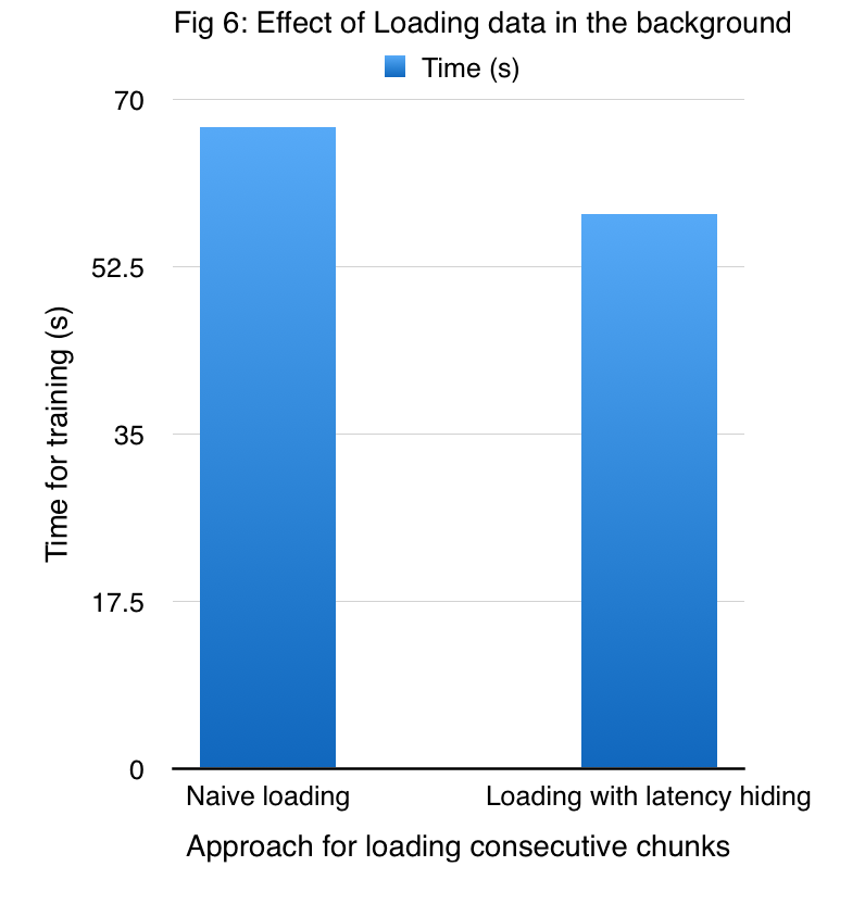
  To hide the latency of reading a shard each time, we implemented a prefetcher, which is responsible for bringing the next chunk of data to host memory, at the time when the device is performing necessary computation with the shard in the device memory. Our prefetcher is a pthread that runs in the background whose primary task is just to read data from disk to DRAM. We thus effectively hide the disk I/O latency by bringing the data in while computations are being performed on the device. We call this the Distributed Approximate Scalable cuGP (DAS-cuGP) approach.

  Figure 6 shows the improved performance due to the prefetcher on a dataset comprising of 24000 points which are divided into 16 shards, while employing 4 GPUs.

  
  

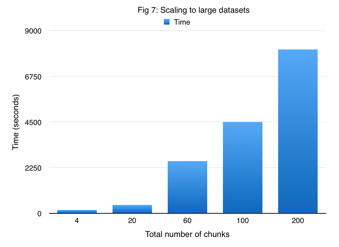
  In order to demonstrate that DAS-cuGP enables us to handle large amounts of data, we applied our method to the US Flight Delay dataset. Given the amount of time for running a job in latedays cluster (3 hours), we subsampled the original data to obtain 1 million samples. There are 7 attributes in the data set which are used to predict the flight arrival delay time. We divide this dataset into 200 shards each having 5000 samples. Figure 7 shows the time required for DAS-cuGP while varying the number of shards. We find that it takes less than 3 hours to do the learning phase in DAS-cuGP for the entire dataset (result corresponding to 200 shards).

  

The Bottom Line

We have written a fast single-GPU implemenation: cuGP for exact GP regression. On comparing its performance with a strong competitive baseline, we find significant speedups for both training as well as prediction phases. Even after searching extensively, we did not find any open source GPU implementation of Gaussian Process Regression, and hence all our benchmarks were compared to our own baselines.

Additionally, we also implemented a recently proposed approximate algorithm for GP regression and tailored it for a distributed multi-GPU environment, thus relaxing the memory requirement for a single GPU exact approach. Our implementation DA-cuGP harnesses the power of multiple GPUs running in parallel. The communication between these GPUs is handled by low-level socket programming. Careful inspection of the individual times suggest that the communication overhead is negligible.

In order to scale to arbitary sized datasets, and to further relax the memory requirement constraint, we have extended the DA-cuGP approach by assigning multiple shards to each GPUs. This implementation, DAS-cuGP, scales well and is able to handle a real world dataset comprising of 1 million input data points.

Work Division

References

[RW06]: Williams, Christopher KI, and Carl Edward Rasmussen. "Gaussian processes for machine learning." the MIT Press 2.3 (2006): 4.

[WN15]: Wilson, Andrew Gordon, and Hannes Nickisch. "Kernel interpolation for scalable structured Gaussian processes (KISS-GP)." arXiv preprint arXiv:1503.01057 (2015).

[DN15]: Deisenroth, Marc Peter, and Jun Wei Ng. "Distributed Gaussian Processes." arXiv preprint arXiv:1502.02843 (2015).

[DA14]: Dong, Tingxing, et al. "A fast batched Cholesky factorization on a GPU." Parallel Processing (ICPP), 2014 43rd International Conference on. IEEE (2014)

[K09]: Knight, Nicholas. "Triangular Matrix Inversion a survey of sequential approaches." (2009).

[RN15]: Rasmussen, Carl Edward, and Hannes Nickisch. "The GPML Toolbox version 3.5." (2015).